Pumas.jl

Pumas: A Pharmaceutical Modeling and Simulation toolkit

Resources

• Downloads & Install Instructions
• Documentation
• Tutorials
• Blog
• Discourse Forum

Demo: A Simple PK model

using Pumas, Plots, LinearAlgebra

For reproducibility, we will set a random seed:

using Random
Random.seed!(1)

A simple one compartment oral absorption model using an analytical solution

model = @model begin
  @param   begin
    tvcl ∈ RealDomain(lower=0)
    tvv ∈ RealDomain(lower=0)
    pmoncl ∈ RealDomain(lower = -0.99)
    Ω ∈ PDiagDomain(2)
    σ_prop ∈ RealDomain(lower=0)
  end

  @random begin
    η ~ MvNormal(Ω)
  end

  @covariates wt isPM

  @pre begin
    CL = tvcl * (1 + pmoncl*isPM) * (wt/70)^0.75 * exp(η[1])
    V  = tvv * (wt/70) * exp(η[2])
  end

  @dynamics ImmediateAbsorptionModel
    #@dynamics begin
    #    Central' =  - (CL/V)*Central
    #end

  @derived begin
      cp = @. 1000*(Central / V)
      dv ~ @. Normal(cp, sqrt(cp^2*σ_prop))
    end
end

Develop a simple dosing regimen for a subject

ev = DosageRegimen(100, time=0, addl=4, ii=24)
s1 = Subject(id=1,  evs=ev, cvs=(isPM=1, wt=70))

Simulate a plasma concentration time profile

param = (
  tvcl = 4.0,
  tvv  = 70,
  pmoncl = -0.7,
  Ω = Diagonal([0.09,0.09]),
  σ_prop = 0.04
  )
obs = simobs(model, s1, param, obstimes=0:1:120)
plot(obs)

Generate a population of subjects

choose_covariates() = (isPM = rand([1, 0]),
              wt = rand(55:80))
pop_with_covariates = Population(map(i -> Subject(id=i, evs=ev, cvs=choose_covariates()),1:10))

Simulate into the population

obs = simobs(model, pop_with_covariates, param, obstimes=0:1:120)

and visualize the output

plot(obs)

Let's roundtrip this simulation to test our estimation routines

simdf = DataFrame(obs)
simdf.cmt .= 1
first(simdf, 6)

Read the data in to Pumas

data = read_pumas(simdf, time=:time,cvs=[:isPM, :wt])

Evaluating the results of a model fit goes through an fit --> infer --> inspect --> validate cycle

fit

julia> res = fit(model,data,param,Pumas.FOCEI())
FittedPumasModel

Successful minimization:                true

Likelihood approximation:        Pumas.FOCEI
Objective function value:            8363.13
Total number of observation records:    1210
Number of active observation records:   1210
Number of subjects:                       10

-----------------
       Estimate
-----------------
tvcl    4.7374
tvv    68.749
pmoncl -0.76408
Ω₁,₁    0.046677
Ω₂,₂    0.024126
σ_prop  0.041206
-----------------

infer

infer provides the model inference

julia> infer(res)
Calculating: variance-covariance matrix. Done.
FittedPumasModelInference

Successful minimization:                true

Likelihood approximation:        Pumas.FOCEI
Objective function value:            8363.13
Total number of observation records:    1210
Number of active observation records:   1210
Number of subjects:                       10

---------------------------------------------------
       Estimate       RSE           95.0% C.I.
---------------------------------------------------
tvcl    4.7374     10.057  [ 3.8036   ;  5.6713  ]
tvv    68.749       5.013  [61.994    ; 75.503   ]
pmoncl -0.76408    -3.9629 [-0.82342  ; -0.70473 ]
Ω₁,₁    0.046677   34.518  [ 0.015098 ;  0.078256]
Ω₂,₂    0.024126   31.967  [ 0.0090104;  0.039243]
σ_prop  0.041206    3.0853 [ 0.038714 ;  0.043698]
---------------------------------------------------

inspect

inspect gives you the model predictions, residuals and Empirical Bayes estimates

resout = DataFrame(inspect(res))

julia> first(resout, 6)
6×13 DataFrame
│ Row │ id     │ time    │ isPM  │ wt    │ pred    │ ipred   │ pred_approx │ wres     │ iwres     │ wres_approx │ ebe_1     │ ebe_2     │ ebes_approx │
│     │ String │ Float64 │ Int64 │ Int64 │ Float64 │ Float64 │ Pumas.FOCEI │ Float64  │ Float64   │ Pumas.FOCEI │ Float64   │ Float64   │ Pumas.FOCEI │
├─────┼────────┼─────────┼───────┼───────┼─────────┼─────────┼─────────────┼──────────┼───────────┼─────────────┼───────────┼───────────┼─────────────┤
│ 1   │ 1      │ 0.0     │ 1     │ 74    │ 1344.63 │ 1679.77 │ FOCEI()     │ 0.273454 │ -0.638544 │ FOCEI()     │ -0.189025 │ -0.199515 │ FOCEI()     │
│ 2   │ 1      │ 0.0     │ 1     │ 74    │ 1344.63 │ 1679.77 │ FOCEI()     │ 0.273454 │ -0.638544 │ FOCEI()     │ -0.189025 │ -0.199515 │ FOCEI()     │
│ 3   │ 1      │ 0.0     │ 1     │ 74    │ 1344.63 │ 1679.77 │ FOCEI()     │ 0.273454 │ -0.638544 │ FOCEI()     │ -0.189025 │ -0.199515 │ FOCEI()     │
│ 4   │ 1      │ 0.0     │ 1     │ 74    │ 1344.63 │ 1679.77 │ FOCEI()     │ 0.273454 │ -0.638544 │ FOCEI()     │ -0.189025 │ -0.199515 │ FOCEI()     │
│ 5   │ 1      │ 0.0     │ 1     │ 74    │ 1344.63 │ 1679.77 │ FOCEI()     │ 0.273454 │ -0.638544 │ FOCEI()     │ -0.189025 │ -0.199515 │ FOCEI()     │
│ 6   │ 1      │ 0.0     │ 1     │ 74    │ 1344.63 │ 1679.77 │ FOCEI()     │ 0.273454 │ -0.638544 │ FOCEI()     │ -0.189025 │ -0.199515 │ FOCEI()     │

validate - vpc

Finally validate your model with a visual predictive check

vpc(res,200) |> plot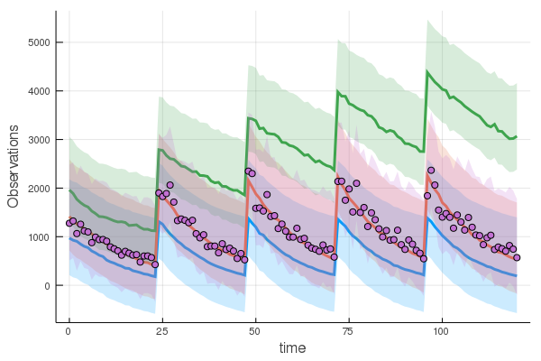

or you can do a vpc into a new design as well.

Plotting methods on model diagnostics are coming soon.

Simulate from fitted model

In order to simulate from a fitted model simobs can be used. The final parameters of the fitted models are available in the res.param

fitparam = res.param

You can then pass these optimized parameters into a simobs call and pass the same dataset or simulate into a different design

ev_sd_high_dose = DosageRegimen(200, time=0, addl=4, ii=48)
s2 = Subject(id=1,  evs=ev_sd_high_dose, cvs=(isPM=1, wt=70))

obs = simobs(model, s2, fitparam, obstimes=0:1:160)
plot(obs)