Implement mixed hmc

[fehiepsi]

Resolves #785.

Tasks

• Implement the core functionality (mimic hmcecs implementation)
• Add an example
• Add tests
  - [ ] Mass adaptation

[fritzo]

(moving conversation from slack)

@fritzo:

Thanks for explaining the M-HMC paper so clearly! Of their experiments, it looks like the GMM and CTR models both have discrete latent variables inside plates with no downstream dependencies outside the plates, therefore you should be able to independently make all reflect/refract decisions in parallel. Their other experiment (variable selection in regression) does not admit the same parallel decision trick though. I can see how they might consider the trick too "model specific", but I'd argue that a PPL like Pyro can automatically detect when the trick is applicable.

@fehiepsi:

Make sense to me. This look like the way we propose a new subsample indices (considering it as an subsample-size discrete variable), i.e. one single clock auxilary variable for that plate-size variable.

Hmm... it seems to be different. It is not clear to me how to make refract/reflex decisions in parallel.

I see your point now. Nice observation!

I think a nice interface to specify this would be to follow the pattern we used for parallel enumeration, where a user could specify an infer config like infer={"enumerate": "sequential"} versus infer={"enumerate": "parallel"}. Thinking about this in more detail, I think we could independently decide whether to parallelize over each of the enclosing plates. So e.g. if we parallelize by default we could specify something a set of enclosing plates outside of which this particular sample site has downstream dependencies (which prevents parallelism), something like infer={"dependent_plates": ["plate1", "plate2"]}.

[fehiepsi]

@fritzo I think it is doable without much change in the implementation. Based on those "infer" information, we can maintain 3 behaviors for a discrete D-size variable x

• D clock positions + D momentum variable, each one corresponding to each item in x: the current implementation
• 1 clock position + D momentum variables for x: this is what you suggested?
• 1 clock position + 1 momentum variable for x: this is useful for a gibbs/subsample update

[fehiepsi]

Hi @StannisZhou, I'm not sure why modified=True is important in case we just take 1 discrete step, but let's just consider that case. For binary distribution, the term Q(x_new)/Q(x) is always 1 in both random walk and Gibbs cases, so the final MH correction always accepts the proposal. This makes the scheme correct. But in cases where the size of the support is >=3, e.g. Binomial(2, 0.8) or Binomial(10, 0.3), the final MH acceptance ratio Q(x_new)/Q(x) will not always be equal to 1 when we use modified Gibbs proposal (random walk proposal is fine).

Another issue is: in Bernoulli(0.8) case, if we take 2 discrete steps, then when we start at the discrete value 1, we will never reach the discrete value 0 because if we accept the proposal in the first step, then discrete kinetic energy will be increased by an amount that always allows us to accept the proposal in the second step. So the chain will stuck at value 1.

[StannisZhou]

Hi @fehiepsi , thanks for bringing up this very important issue. I still need to look a bit more into this, but a few points I know at the moment:

1. My memory was a bit fuzzy since It has been a while, but if you look at Algorithm 1 on page 3 of my original discrete only formulation, you can see that there was no final MH correction. And it makes sense since in the discrete only case, the integration of the Hamiltonian dynamics is exact, and no correction is needed. This would resolve your failing tests, and all the points you raised (since mixed HMC reduces to a regular MH update in such cases). I revised my earlier comment to reflect this point.
2. The acceptance ratio you gave (p(x_new) / p(x) * [p(x_new) / p(x) * Q(x) / Q(x_new)] = p^2(x_new) / p^2(x) * Q(x) / Q(x_new)) does not seem to be consistent with what I have in the paper. In my terminology, the log acceptance ratio is -(E-E_0) (line 10 Algorithm 1). In the discrete only case you mentioned, E=U + k_0 - \Delta E, and E_0 = U_0 + k_0, and \Delta E = U - U_0 + log Q(x|x_0) - log Q(x_0|x) (line 19 of Algorithm 1), so the log acceptance ratio is -[U - U_0 - (U - U_0 + log Q(x|x_0) - log Q(x_0|x))] = log Q(x|x_0) - log Q(x_0|x). In your terminology, the acceptance ratio should actually be p(x_new) / p(x) * [p(x) / p(x_new) * Q(x_new) / Q(x)] = Q(x_new) / Q(x). For random walk proposals this ratio is always 1. So if you fix the acceptance ratio your tests shouldn't be failing for random walk proposals.
3. Although for random walk proposals it works, the remaining log Q(x|x_0) - log Q(x_0 | x) term still looking problematic, and would break non-random walk proposals. It should be naturally 0 for such cases. I'm still looking into this. I have some hypotheses, and I think there's a chance you actually helped me find the simpler formulation I've been trying (but failing) to get, although there might also be mess-ups in my current formulation (but fortunately it seems numerical results are fine). Will keep you posted.

[fehiepsi]

the acceptance ratio should actually be p(x_new) / p(x) * [p(x) / p(x_new) * Q(x_new) / Q(x)] = Q(x_new) / Q(x). For random walk proposals this ratio is always 1. So if you fix the acceptance ratio your tests shouldn't be failing for random walk proposals

Agreed! The formula p^2(x_new) ... is used for not-modified Gibbs case, where Q(x_new)/Q(x) = p(x_new)/p(x). And as I mentioned in my last comment, the scheme is fine for binary distributions or higher support size distributions with modified/not-modified random walk proposals. It will likely cause issues for not-modified Gibbs proposal in general or for modified Gibbs proposal with support size >= 3.

About the tests, I believe if I add an independent continuous variable to the model that has an exact HMC dynamics, the tests will fail by the same reason. On the other hand, tests are aslo failing because the periodicity that I mentioned in my last comment: if we use the scheme (with/without the final MH correction) for Bernoulli(0.8) with 2 discrete updates per each MCMC step, the chain will stuck at value 1.

About a simpler formulation, we mimiced the scheme in your paper but separating out the HMC halminton dynamics and discrete halmintonian dynamics. In other words, we consider the continuous variable as a discrete variable and HMC dynamics with MH proposal as a Gibbs proposal (i.e. Delta_E = 0). That way, we don't need the final MH correction and it allows us to use the full NUTS update each time we want to update the continuous variable. We are still making the mass adaptation scheme (to control the speed of updates) to be more polished to be able to deliver it to users. Without mass adaptation, the scheme will be similar to random Gibbs scan as you mentioned.

[StannisZhou]

Agreed about the periodicity case. I basically made a technical assumption when proving correctness.

Your comments led me to think there might be mess-ups in my cancellation reasonings in the proof which led to the seemingly incorrect final correction. I'm looking into this point.

I see your point about taking the continuous part as a discrete variable. That's very interesting, and sounds similar but slightly different from what I'm thinking (and what I had in the paper). To make sure I understand, you specify an auxiliary kinetic energy for the continuous part of the system, then after each continuous Hamiltonian dynamics step you calculate the energy difference and decide whether you accept/reject based on whether you have enough kinetic energy?

[fehiepsi]

Yes, that is similar to a sequence of Gibbs updates in MH-within-Gibbs, but updating (not reseting) the kinetic energy each time we update a variable, as in your paper. We just found that the scheme makes it easier to adjust the selection probability for which variable we want to update each time (e.g. some variables we want to update more often than the others). There are other ways to adjust the selection probabilty but the scheme in your paper is more intuitive to me.

In NUTS (and HMC with MH correction too), the accept ratio (after all internal MH corrections in HMC/NUTS) will always be 1, so having an auxiliary kinetic energy is not important. But it is good to use your scheme (with constant kinetic energy) to adjust the speed, hence we can adapt for how often we want to perform NUTS update in an MCMC step.

[StannisZhou]

So you are indeed making an MH correction after each continuous HMC update. I don't think that's necessarily the best scheme in the HMC case, but for NUTS it does make more sense.

[fehiepsi]

Updated: by incoporating the updated version by @StannisZhou, tests pass now. The new formula has the last acceptance ratio = 1 when the continuous HMC dynamic is exact - so it looks more reasonable than previously.

[StannisZhou]

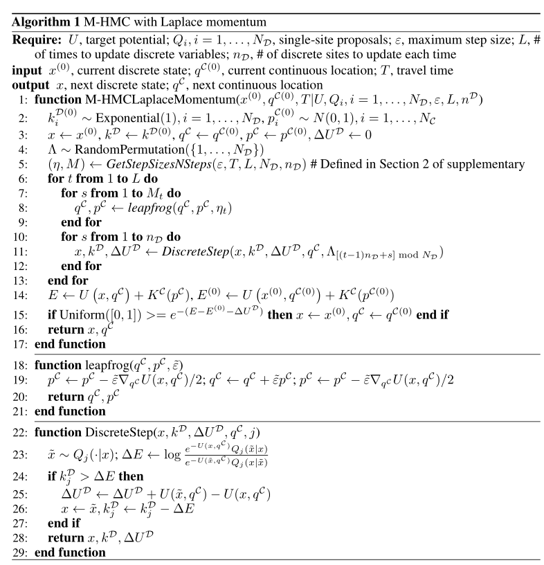
Thanks @fehiepsi ! I'm attaching the updated algorithm as reference while I'm working to fix the MH term in the paper.
.

[StannisZhou]

Update: I have fixed the arxiv version of the paper and the code on github. I additionally included a script to showcase sampling with different proposal distributions (e.g. Gibbs proposals which were invalid with previous MH correction).

A brief postmortem:

1. The mistake was in Lemma 4 in supplementary, and was introduced when I adapted the proof from discrete-only case to mixed discrete and continuous case. I have fixed the proof and included (previously omitted) detailed intermediate calculations.
2. The initial incorrect MH correction is the same as the correct one when we use (modified or not) random-walk proposals and for modified proposals on binary variables. In addition, for models where there are at most 2 nonzero entries in conditional distributions (e.g. the 1D GMM example I used, where components are well separated), previous MH correction with modified Gibbs is indistinguishable from the correct MH correction (previous delta_E = log(1 - p_new) - log(1 - p) \approx log(p) - log(p_new) = U_new - U = new delta_U). These happen to cover all my experiments and sanity checks (mostly on GMM and to a less degree on BLR) so I didn't spot the error from the numerical experiments.

Also see the erratum for more details and some additional experiments on performances of mixed HMC with different discrete proposals.

[martinjankowiak]

great to hear. thanks @StannisZhou for following up!

[fehiepsi]

Thanks for reviewing and feedback, @martinjankowiak and @StannisZhou!