When driving a car, a human being is, without even noticing, submitted to an infinity of factors that requires its constant attention and focus, like observing the other cars on his/her surroundings, being careful about pedestrians crossing the road, and even having to constantly observe the lane lines to make sure that the car is rightly positioned on the track.
Because these perceptions may be such an intrinsic task for us, we often realize them even without noticing. But, how could a computer detect and identify lane lines on a road, for example? In this project, as part of the first module of Udacity`s Self Driving Car Nanodegree, I'll be exploring and explaining the pipeline used to make an algorithm that, using Python and Computer Vision, can identify lane lines on multiple static images and videos (which are, really, just a bunch of images together).
The lane lines detector algorithm is basically consisted of X steps:
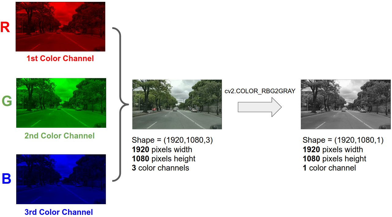
- Convert the image's color-space from RGB to Grayscale
- Apply a Gaussian Blur to the Grayscale Image
- Apply a Canny Filter for Edge Detection
- Define the 'Region of Interest'
- Draw lines with Hough Space
- Combine the algorithm's drawn lines with the original image, so we can see the highlighted lines in real time
RGB Color images have, as the name suggests, 3 color channels (Red, Green and Blue). Before applying the Canny Filter for edge detection, one technique that can be applied in order to use less computational power is to transform the 3-Color-Channel RGB image into a 1-Color-Channel Grayscale image, so the process become less computational intensive and even faster!
img_gray = cv2.imread(‘Image_location_path’
cv2.IMREAD_GRAYSCALE)
plt.imshow(img_gray, cmap=’gray’) # We have to change the cmap because of the standard
#blue-green color map that matplotlib uses as standard.
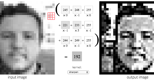
A common operation for image processing is blurring (or smoothing) an image. Blurring an image helps to reduce the noise and helps an application focus on general details. Kernels-Based Filters can be applied over an image to produce a variety of effects. E.g. Basically, a kernel is a matrix, and, for each 3x3 block of pixels in the image, we multiply each by the corresponding entry of the kernel and then take the sum. That sum becomes a new pixel in the new image.
blur_image = gaussian_blur(img=gray_image, kernel_size=5)
plt.imshow(blur_image, cmap='gray')
Used to identify sharp changes in intensity in adjacent pixels, the Canny Edge Detector algorithm is a tool that identifies points in a digital image at which the image brightness changes sharply or has discontinuities.

Developed in 1986 by John Canny, the Canny Edge detector is considered a multi-stage algorithm, composed of the following stages:
- Apply a Gaussian filter to smooth the image in order to remove the noise, once noise can create false edges and affect the edge detection algorithm. Obs: you may want to apply your own blur/smooth filter before the one that comes with Canny, in case your image has too many features and high resolution).
- Find the intensity gradients of the image.
- Apply non-maximum suppression to get rid of spurious response to edge detection.
- Apply a double threshold to determine potential edges.
- Track edge by hysteresis: Finalize the detection of edges by suppressing all the other edges that are weak and not connected to strong edges (In other words, it gets rid of weak edges and only keep the strong ones).

In this lane lines case, we get the following result:

median_pixel_value = np.median(blur_image)
lower_threshold = int(max(0, 0.7*median_pixel_value))
upper_threshold = int(min(255, 1.3*median_pixel_value))
canny_image = canny(img=blur_image, low_threshold=lower_threshold, high_threshold=upper_threshold)
plt.imshow(canny_image, cmap='gray')
Ps: Read more about Canny Edge Detector here and here.
In order to only apply the Hough Transform on the region we actually are interested on (which is, obviously, on the lane lines region!) and achieve better results, we must create a mask show only our region of interest to the Hough Transform algorighm, in the pipeline next step.
To do so, it is needed to create a completely blank image with the same size of out original image, and then create a white polygon that involves the area we want to mask (where black is represented by 0 or 00000000 and white is represented by 255 or 11111111).

def region_of_interest(image):
 height = image.shape[0]
	width = image.shape[1]
	#Because of the function “fillPoly”, we must specify an array of several polygons.
	#In this case, is just one triangle
	polygons = np.array([
	[(200, height), (1100, height), (550, 250)]
 	   ^              ^               ^    ^
	])
	black_mask = np.zeros_like(image)
	cv2.fillPoly(black_mask, polygons, color=255)
return black_mask
To effectvelly apply the mask to the image, a bitwise "&" operation is used. By doing that, because the fact that both the mask image and the lane_image have the same array shape (consequently, the same dimensions / the same amount of pixels), only the white pixels on both images will be shown. This happens because, in the bitwise &, a black pixel (0000) will always result in black (0000) and a white pixel (1111) will always result in the first factor of the operation (in other words, it will always be equal to the white or black inicial image, it will have no effect on the image masked image).

masked_image = cv2.bitwise_and(src1 = image, src2 = black_mask)
Here is an example of the mask application on a video I recorded:

The technique used to detect straight lines on the image and thus identify the main line is known as Hough Transform.
Basically, a parametric space of b x m (from y = mx + b) is called Hough Space. As we can see in the image, the yellow point in xy can be represented by a line in bm. In the same way, the purple line in xy can be represented by a point in bm. So, to draw a line, we take the intersection point of the lines in bxm and draw a line in our image using the formed equation.

But first, we need to use polar coordinates instead of cartesian coordinates. The more curves intersecting, it means that the line created by that intersection crosses more points, and the line generated in our image will be more precise!

Our drawn line will be equal to the bin point that has more votes - the one that has more intersections on it. The larger the bins, the less precision our lines are going to be detected. The smaller the ro and degree intervals, bigger will be the precision. But we don't want them to be too small or it will take more time to process and run.

Ps: More reference to study about hough transform here.
lines = cv2.HoughLinesP(img=cropped_img,  rho = 2 , theta = np.pi/180), threshold=100)
                                             ^           ^
                              Precision in pixels   Degree precision in radians
# Here, the threshold is the minimum number of votes needed to accept a candidate line.
# So, in this case, the minimum number of intersections need to be at least 100 to be accepted as
# a relevant line to describe our data.

To optimize how the lines are displayed (instead of having multiple lines, we will average them to become a single line that intercept the entire lane in our lane_image) we use:
def average_slope_intercept(img, lines):
	#left_fit contains the coordinates of the averaged lines on the left and
	#right_fit contains the coordinates of the averaged lines on the right
	left_fit    = []
	right_fit   = []
	if lines is None:
    		return None
	for line in lines:
    	for x1, y1, x2, y2 in line:
        	fit = np.polyfit(x=(x1,x2), y=(y1,y2), deg=1)
        	slope = fit[0]
        	intercept = fit[1]
        	# According to the cartesian coordinates and the equation y = mx+b,
        	# if the slope is negative, it belongs to the left line (because the values of y are decreasing)
        	# and if slope is positive, it belongs to the right line
        	if slope < 0: # y is reversed in image
           		left_fit.append((slope, intercept))
        	else:
           		right_fit.append((slope, intercept))
	# add more weight to longer lines
	if len(left_fit) and len(right_fit):
    	left_fit_average  = np.average(left_fit, axis=0)
    	right_fit_average = np.average(right_fit, axis=0)
    	left_line  = make_points(image, left_fit_average)
    	right_line = make_points(image, right_fit_average)
    	averaged_lines = [left_line, right_line]
    	return averaged_lines

Ps: In order to better understand the parameter tuning, we can also use this GUI helper tool.
As we can see, the hough_lines function's output is a black image with the red lines on it. In order to better visualize the lane lines identification, it is needed to combine both the lines and the original image.
combined_image = weighted_img(img=line_image, initial_img=image, α=0.8, β=1., γ=0.)
plt.imshow(combined_image)

So, the final result for multiple static images was pretty decent, as we can see on the image bellow:

One shortcoming observed during the algorithm test on the video was that, in some cases, the projected lane lines were not stable - they were blinking.

To solve this blinking issue, I followed the mentor's hint (found in this question's answer), and tuned the parameters to optimize the line detection, where, according to the mentor:
-
max_line_gap that defines the maximum distance between segments that will be connected to a single line.
-
min_line_len that defines the minimum length of a line that will be created. Increasing min_line_lenand max_line_gap(~100 and above) for Hough Transform will make your lines longer and will have less number of breaks.(this will make the solid annotated line longer in the output)Increasing max_line_gap will allow points that are farther away from each other to be connected with a single line.
-
threshold increasing (~ 50-60) will rule out the spurious lines.(defines the minimum number of intersections in a given grid cell that are required to choose a line.)
-
Decreasing the kernel-size in the Gaussian Filter might also help, as this will remove the noise making the image less blurry.
-
Consider using rho value of 2 ( rho, distance resolution of the Hough accumulator in pixels.)
-
The detection of straight edges through Hough transform will induce some uncertainties because of the variations in the photograph conditions such as lighting, shadow, vibrations etc. This makes the calculations of the slopes and the end points fluctuate within a certain zone. In order to avoid this noise, a Kalman filter can also be used to smoothen out the fluctuations in the slope and end point estimation.
And the result became:

So, for future projects, it may be needed to tune these parameters again, to get optimum lane detection depending on the new video condition.
I have no doubts that this pipeline can (and will!) be improved in the future. Personally speaking, I still want to study deeply the Hough Lines / Hough Transform algorithm, once it seems to be a very interesting and complex field to study. As it is possible to see on the lane lines detection gif above, we can see that the lane lines are not completely static - they are shaking a little bit and can be improved.